How I turned famous paintings into pie chart graphs

Every painting tells a story through color. But what does that story look like as data? I made a Python script to extract the 7 dominant colors from famous paintings using machine learning and visualized the results as pie charts.

Here's how it works, what I learned, and the full code so you can try it yourself.‍

The Results

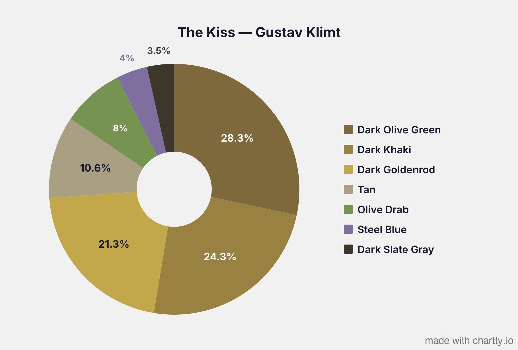
Klimt - The Kiss is 74% gold

‍

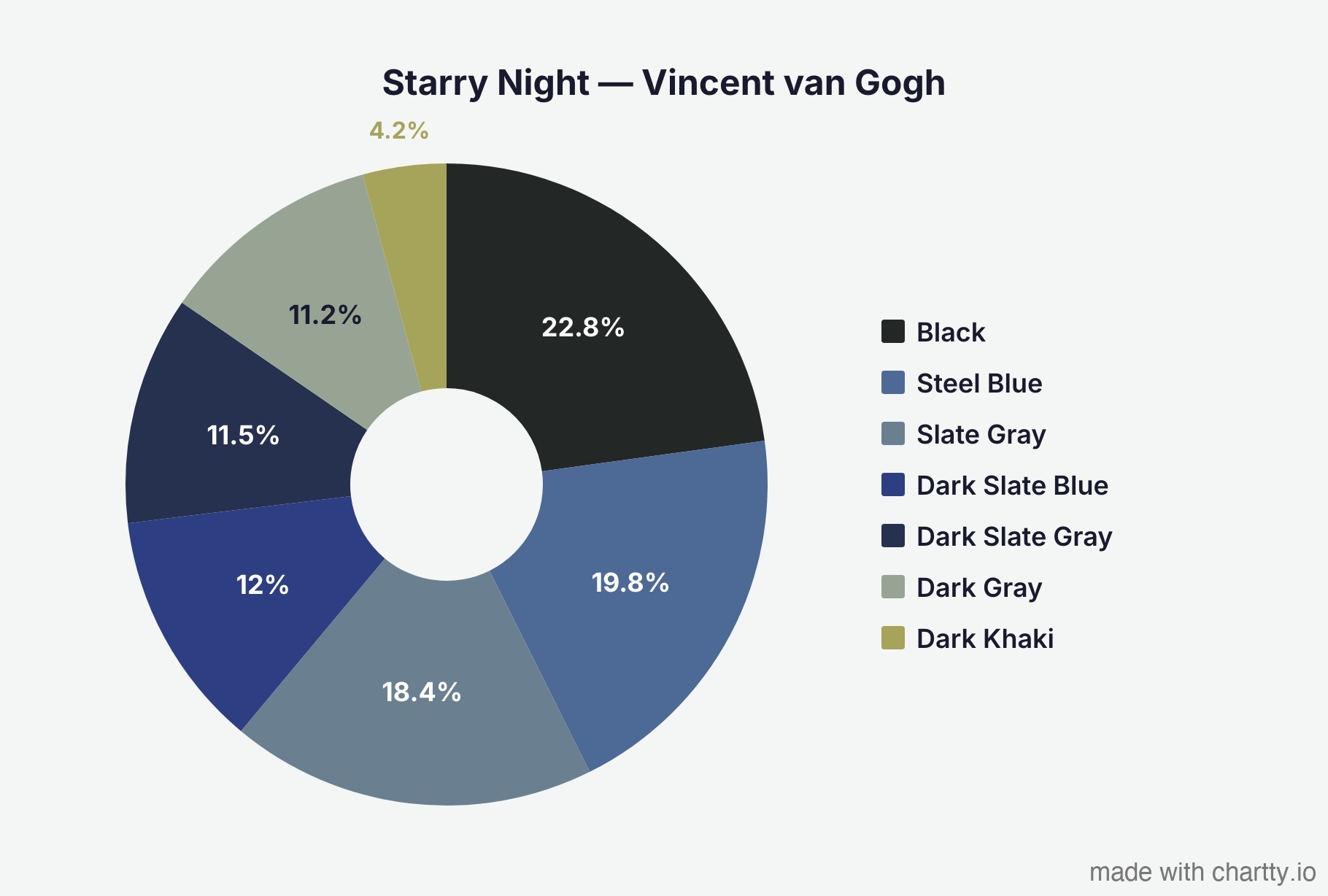
Van Gogh's - Starry Night is overwhelmingly blue.

‍

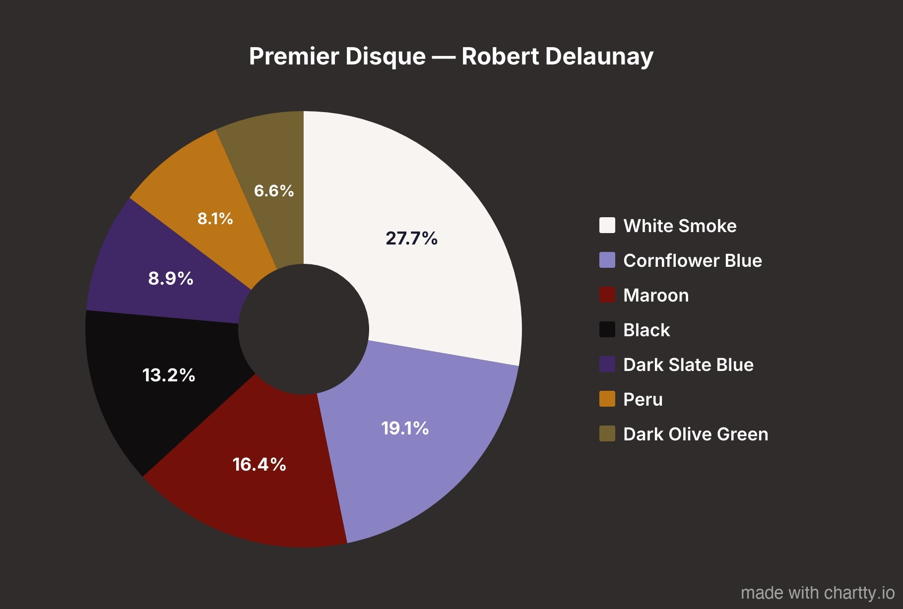
Delaunay's - Premier Disque is the most evenly distributed palette.

‍

Matisse's Fauvist masterpiece shows why the critics were scandalized.

‍

The Scream is warmer than you'd expect.

‍

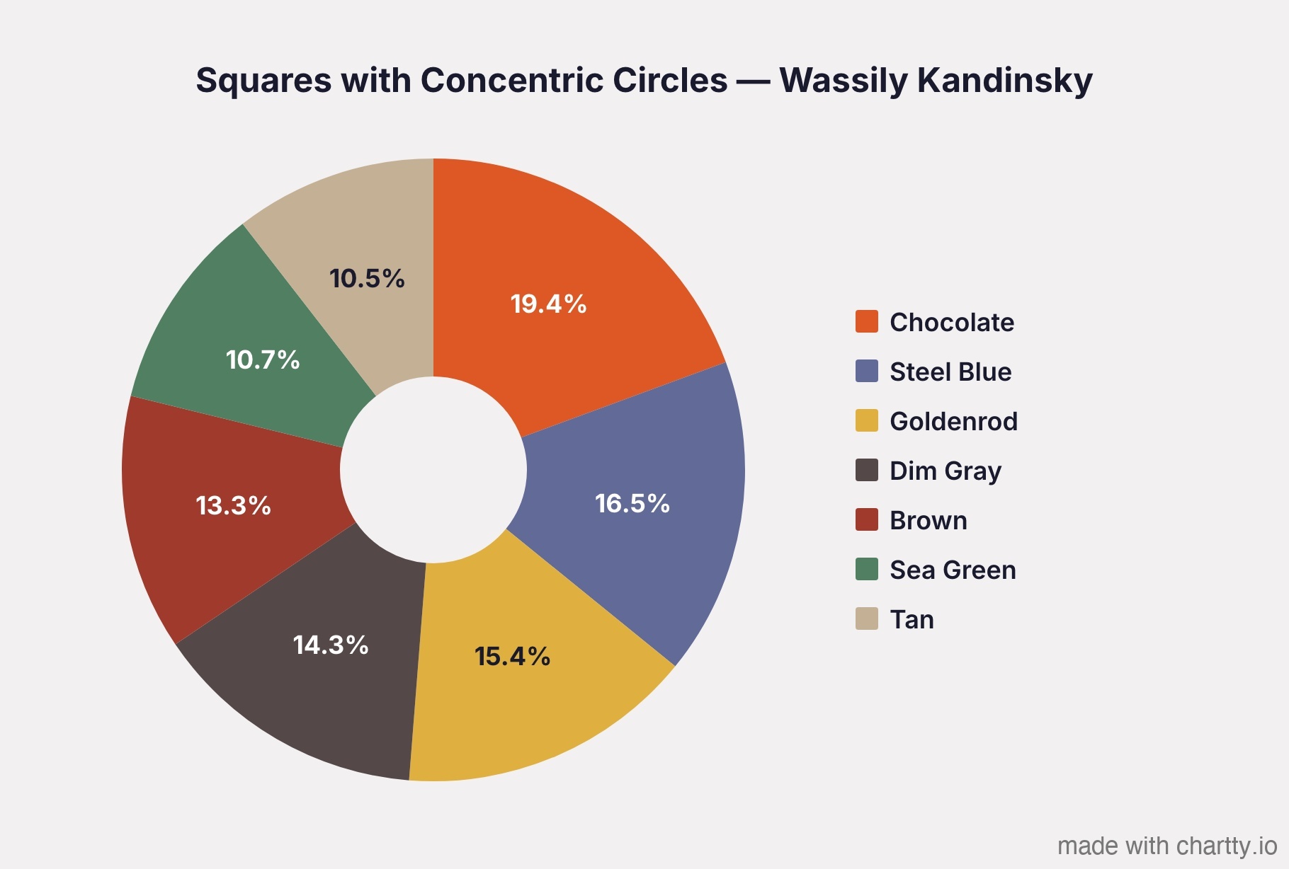
Kandinsky's color study is the most balanced. No single color dominates.

The Method: Why Most Color Extraction is Wrong

If you Google "extract colors from image Python," most tutorials will tell you to run K-means clustering on the RGB pixel values. This works, but it has a bias: RGB space is not perceptually uniform.

What does that mean? In RGB, the Euclidean distance between two colors doesn't correspond to how different those colors look to a human eye. Dark tones occupy a disproportionately large volume of RGB space, so K-means clusters tend to skew darker than the painting actually appears.

The fix: cluster in CIELAB color space instead

CIELAB was designed by the CIE specifically so that equal distances in the space correspond to equal perceived color differences. The L channel is perceptual lightness, A is green-to-red, and B is blue-to-yellow. When you run K-means in CIELAB, the clusters represent perceptually meaningful groups of color.

Here's the pipeline:

Painting image (RGB pixels)

 → Convert to CIELAB color space

 → K-means clustering (7 clusters)

 → Convert cluster centers back to RGB

 → Map each center to nearest CSS named color

 → Generate pie chart

Why CIELAB matters: a real example

When I first ran this on Munch's The Scream using standard RGB clustering, the warm orange sky got absorbed into nearby dark clusters, making the painting look almost entirely gray-brown.

Switching to CIELAB gave the warm tones their own clusters because CIELAB treats perceived color differences equally regardless of lightness.

Why CSS named colors?

Early versions of the script used hand-tuned color names based on HSV thresholds, things like "Dusty Amber" and "Light Azure." People rightfully pointed out that these names are meaningless. Who knows what "Dusty Amber" is?

Instead, I map each extracted color to the nearest of the 148 standard CSS named colors using Delta E distance in CIELAB. Everyone knows what "Steel Blue" or "Sienna" looks like. The naming becomes objective and reproducible, it's just "which CSS color is closest in perceptual space?"

When two segments map to the same CSS color, the script finds the next-closest unused CSS color instead, so every label in a chart is unique.

The Code

Full script below. Requires

pip install pillow numpy scikit-learn requests.

Add paintings to the PAINTINGS list and run python analyze_paintings.py. It downloads each image, runs the analysis, and saves pie chart data you can plug into any charting tool.

python
import numpy as np
from PIL import Image
from sklearn.cluster import KMeans
import requests
import io

N_COLORS = 7

# ── CIELAB conversion ──────────────────────────────────────────

def rgb_to_lab_batch(rgb):
    """Convert Nx3 RGB (0-255) array to CIELAB (D65 illuminant)."""
    rgb_norm = rgb / 255.0
    mask = rgb_norm > 0.04045
    linear = np.where(mask, ((rgb_norm + 0.055) / 1.055) ** 2.4, rgb_norm / 12.92)

    r, g, b = linear[:, 0], linear[:, 1], linear[:, 2]
    x = (r * 0.4124564 + g * 0.3575761 + b * 0.1804375) / 0.95047
    y = (r * 0.2126729 + g * 0.7151522 + b * 0.0721750)
    z = (r * 0.0193339 + g * 0.1191920 + b * 0.9503041) / 1.08883

    def f(t):
        return np.where(t > 0.008856, np.cbrt(t), (903.3 * t + 16) / 116)

    fx, fy, fz = f(x), f(y), f(z)
    return np.column_stack([116 * fy - 16, 500 * (fx - fy), 200 * (fy - fz)])


def lab_to_rgb(lab):
    """Convert Nx3 CIELAB back to RGB (0-255)."""
    L, a, b_lab = lab[:, 0], lab[:, 1], lab[:, 2]
    fy = (L + 16) / 116
    fx, fz = a / 500 + fy, fy - b_lab / 200

    def f_inv(t):
        t3 = t ** 3
        return np.where(t3 > 0.008856, t3, (116 * t - 16) / 903.3)

    x = f_inv(fx) * 0.95047
    y = f_inv(fy)
    z = f_inv(fz) * 1.08883

    r = x *  3.2404542 + y * -1.5371385 + z * -0.4985314
    g = x * -0.9692660 + y *  1.8760108 + z *  0.0415560
    b = x *  0.0556434 + y * -0.2040259 + z *  1.0572252

    def gamma(c):
        return np.where(c > 0.0031308, 1.055 * np.power(np.maximum(c, 0), 1/2.4) - 0.055, 12.92 * c)

    return np.clip(np.column_stack([gamma(r), gamma(g), gamma(b)]) * 255, 0, 255).astype(int)


# ── CSS named colors (148 standard) ───────────────────────────

CSS_COLORS = {
    "AliceBlue": (240,248,255), "AntiqueWhite": (250,235,215), "Aquamarine": (127,255,212),
    "Beige": (245,245,220), "Bisque": (255,228,196), "Black": (0,0,0),
    "Blue": (0,0,255), "BlueViolet": (138,43,226), "Brown": (165,42,42),
    "BurlyWood": (222,184,135), "CadetBlue": (95,158,160), "Chartreuse": (127,255,0),
    "Chocolate": (210,105,30), "Coral": (255,127,80), "CornflowerBlue": (100,149,237),
    "Cornsilk": (255,248,220), "Crimson": (220,20,60), "Cyan": (0,255,255),
    "DarkBlue": (0,0,139), "DarkCyan": (0,139,139), "DarkGoldenrod": (184,134,11),
    "DarkGray": (169,169,169), "DarkGreen": (0,100,0), "DarkKhaki": (189,183,107),
    "DarkMagenta": (139,0,139), "DarkOliveGreen": (85,107,47), "DarkOrange": (255,140,0),
    "DarkOrchid": (153,50,204), "DarkRed": (139,0,0), "DarkSalmon": (233,150,122),
    "DarkSeaGreen": (143,175,143), "DarkSlateBlue": (72,61,139),
    "DarkSlateGray": (47,79,79), "DarkTurquoise": (0,206,209), "DarkViolet": (148,0,211),
    "DeepPink": (255,20,147), "DeepSkyBlue": (0,191,255), "DimGray": (105,105,105),
    "DodgerBlue": (30,144,255), "Firebrick": (178,34,34), "ForestGreen": (34,139,34),
    "Gainsboro": (220,220,220), "Gold": (255,215,0), "Goldenrod": (218,165,32),
    "Gray": (128,128,128), "Green": (0,128,0), "HotPink": (255,105,180),
    "IndianRed": (205,92,92), "Indigo": (75,0,130), "Ivory": (255,255,240),
    "Khaki": (240,230,140), "Lavender": (230,230,250), "LightBlue": (173,216,230),
    "LightCoral": (240,128,128), "LightGray": (211,211,211), "LightGreen": (144,238,144),
    "LightPink": (255,182,193), "LightSalmon": (255,160,122),
    "LightSeaGreen": (32,178,170), "LightSkyBlue": (135,206,250),
    "LightSlateGray": (119,136,153), "LightSteelBlue": (176,196,222),
    "Linen": (250,240,230), "Magenta": (255,0,255), "Maroon": (128,0,0),
    "MediumAquamarine": (102,205,170), "MediumBlue": (0,0,205),
    "MediumOrchid": (186,85,211), "MediumPurple": (147,112,219),
    "MediumSeaGreen": (60,179,113), "MediumSlateBlue": (123,104,238),
    "MediumTurquoise": (72,209,204), "MediumVioletRed": (199,21,133),
    "MidnightBlue": (25,25,112), "Moccasin": (255,228,181),
    "NavajoWhite": (255,222,173), "Navy": (0,0,128), "OldLace": (253,245,230),
    "Olive": (128,128,0), "OliveDrab": (107,142,35), "Orange": (255,165,0),
    "OrangeRed": (255,69,0), "Orchid": (218,112,214), "PaleGoldenrod": (238,232,170),
    "PaleGreen": (152,251,152), "PaleTurquoise": (175,238,238),
    "PaleVioletRed": (219,112,147), "PapayaWhip": (255,239,213),
    "PeachPuff": (255,218,185), "Peru": (205,133,63), "Pink": (255,192,203),
    "Plum": (221,160,221), "PowderBlue": (176,224,230), "Purple": (128,0,128),
    "Red": (255,0,0), "RosyBrown": (188,143,143), "RoyalBlue": (65,105,225),
    "SaddleBrown": (139,69,19), "Salmon": (250,128,114), "SandyBrown": (244,164,96),
    "SeaGreen": (46,139,87), "Sienna": (160,82,45), "Silver": (192,192,192),
    "SkyBlue": (135,206,235), "SlateBlue": (106,90,205), "SlateGray": (112,128,144),
    "Snow": (255,250,250), "SteelBlue": (70,130,180), "Tan": (210,180,140),
    "Teal": (0,128,128), "Thistle": (216,191,216), "Tomato": (255,99,71),
    "Turquoise": (64,224,208), "Violet": (238,130,238), "Wheat": (245,222,179),
    "White": (255,255,255), "WhiteSmoke": (245,245,245), "Yellow": (255,255,0),
    "YellowGreen": (154,205,50),
}

# Pre-compute CSS color positions in LAB space
_css_names = list(CSS_COLORS.keys())
_css_labs = rgb_to_lab_batch(np.array([CSS_COLORS[n] for n in _css_names], dtype=float))


def nearest_css_name(rgb):
    """Find the closest CSS color name using Delta E in CIELAB."""
    lab = rgb_to_lab_batch(np.array([rgb], dtype=float))[0]
    distances = np.sqrt(np.sum((_css_labs - lab) ** 2, axis=1))
    name = _css_names[np.argmin(distances)]
    # "DarkSlateGray" -> "Dark Slate Gray"
    return ''.join(f' {c}' if c.isupper() and i > 0 else c for i, c in enumerate(name)).strip()


# ── Main analysis ─────────────────────────────────────────────

def analyze_painting(image_path_or_url, n_colors=N_COLORS):
    """Extract dominant colors from a painting image.

    Args:
        image_path_or_url: Local file path or URL to the painting image.
        n_colors: Number of color clusters (default 7).

    Returns:
        List of dicts with keys: name, hex, rgb, percentage
    """
    if image_path_or_url.startswith("http"):
        headers = {"User-Agent": "ColorAnalysis/1.0"}
        response = requests.get(image_path_or_url, headers=headers, timeout=30)
        response.raise_for_status()
        img = Image.open(io.BytesIO(response.content)).convert("RGB")
    else:
        img = Image.open(image_path_or_url).convert("RGB")

    # Resize for performance (800px preserves enough detail)
    img.thumbnail((800, 800))
    pixels_rgb = np.array(img).reshape(-1, 3).astype(float)

    # Cluster in CIELAB for perceptual uniformity
    pixels_lab = rgb_to_lab_batch(pixels_rgb)
    kmeans = KMeans(n_clusters=n_colors, random_state=42, n_init=10)
    kmeans.fit(pixels_lab)

    labels, counts = np.unique(kmeans.labels_, return_counts=True)
    total = counts.sum()
    centers_rgb = lab_to_rgb(kmeans.cluster_centers_)

    # Build results, sorted by dominance
    colors = []
    used_names = set()
    for i in np.argsort(-counts):
        rgb = tuple(centers_rgb[i])
        pct = round(counts[i] / total * 100, 1)

        # Find unique CSS color name
        lab = rgb_to_lab_batch(np.array([rgb], dtype=float))[0]
        distances = np.sqrt(np.sum((_css_labs - lab) ** 2, axis=1))
        for idx in np.argsort(distances):
            name = _css_names[idx]
            spaced = ''.join(f' {c}' if c.isupper() and j > 0 else c for j, c in enumerate(name)).strip()
            if spaced not in used_names:
                used_names.add(spaced)
                break

        colors.append({
            "name": spaced,
            "hex": "#{:02x}{:02x}{:02x}".format(*rgb),
            "rgb": rgb,
            "percentage": pct,
        })

    return colors


# ── Example usage ─────────────────────────────────────────────

if __name__ == "__main__":
    PAINTINGS = [
        ("The Kiss", "Gustav Klimt",
         "https://upload.wikimedia.org/wikipedia/commons/4/40/The_Kiss_-_Gustav_Klimt_-_Google_Cultural_Institute.jpg"),
        ("The Scream", "Edvard Munch",
         "https://upload.wikimedia.org/wikipedia/commons/c/c5/Edvard_Munch%2C_1893%2C_The_Scream%2C_oil%2C_tempera_and_pastel_on_cardboard%2C_91_x_73_cm%2C_National_Gallery_of_Norway.jpg"),
        ("Squares with Concentric Circles", "Wassily Kandinsky",
         "https://upload.wikimedia.org/wikipedia/commons/9/98/Vassily_Kandinsky%2C_1913_-_Color_Study%2C_Squares_with_Concentric_Circles.jpg"),
    ]

    for name, artist, url in PAINTINGS:
        print(f"\n{'='*60}")
        print(f"{name} — {artist}")
        print(f"{'='*60}")
        colors = analyze_painting(url)
        for c in colors:
            print(f"  {c['percentage']:5.1f}%  {c['hex']}  {c['name']}")

Running it

bash
pip install pillow numpy scikit-learn requests
python analyze_paintings.py
```

Output:

```
============================================================
The Kiss — Gustav Klimt
============================================================
  28.3%  #7d693b  Dark Olive Green
  24.3%  #998141  Dark Khaki
  21.3%  #c2a84a  Dark Goldenrod
  10.6%  #a99f82  Tan
   8.0%  #779352  Olive Drab
   4.0%  #7f6f9f  Steel Blue
   3.5%  #3e362b  Dark Slate Gray

‍

Make a pie chart

To generate the actual pie charts, I plugged the data into Chartty, a pie chart maker, and exported them as JPEGs.